ซ่อนค่าซ้ำใน Excel เหลือไว้ตัวแรก ไม่ต้องใช้ตัวอักษรสีขาว
Hide Repeated Values in Excel – Keep the First One, No White Font
THทริคนี้ทำให้ค่าที่ซ้ำกับแถวบนมองไม่เห็น แต่ข้อมูลยังอยู่ครบ ใช้ได้กับพื้นทุกสี
ENThis trick hides values that repeat the row above. The data is still there. It works on any background colour.
1. ปัญหาที่ผมเจอ | The Problem
THผมจดงานประจำวันใน Excel วันหนึ่งมีหลายแถว วันที่เลยซ้ำกันเต็มคอลัมน์ ดูแล้วลายตา
ผมหาวิธีซ่อนวันที่ซ้ำอยู่นาน เจอแต่วิธี "เปลี่ยนตัวอักษรเป็นสีขาว"
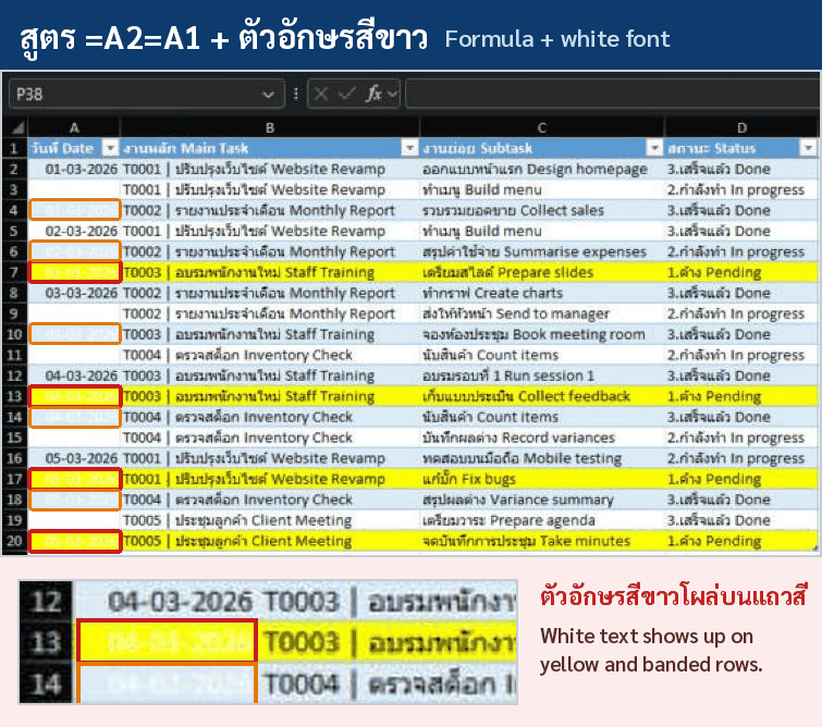
วิธีนี้ใช้ได้แค่ตอนพื้นเป็นสีขาว พอตารางมีแถวสลับสี หรือมีแถวที่ไฮไลต์ไว้ ตัวอักษรสีขาวก็โผล่ให้เห็น
วิธีที่ได้ผลจริงคือ ใช้รูปแบบตัวเลข ;;; ใน Conditional Formatting วิธีนี้ไม่ต้องยุ่งกับสีเลย
ENI keep a daily work log in Excel. Each day has several rows, so the Date column is full of repeats. It's hard to read.
I searched for a long time. Every tip said "make the font white". That only works on a white background.
On banded rows or highlighted rows, the white text shows up.
What actually works is a ;;; number format inside Conditional Formatting. No colours needed.
2. ก่อน / หลัง | Before / After
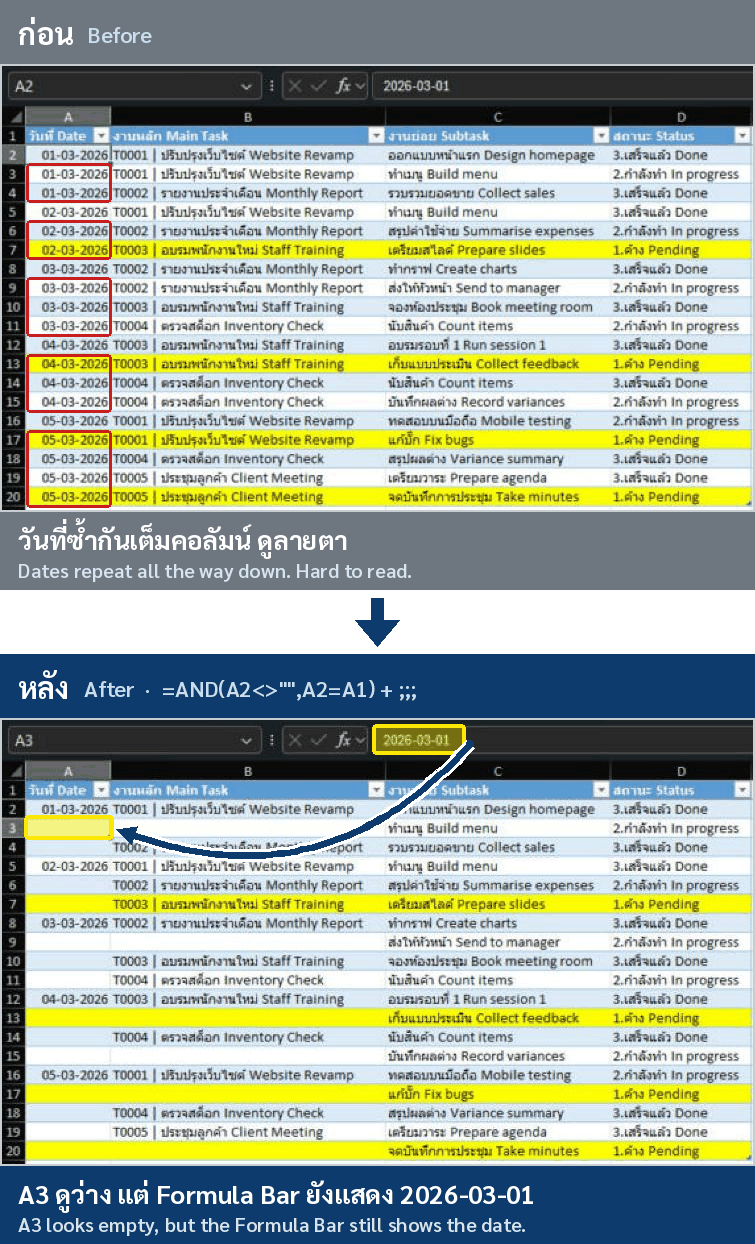
ก่อน | Before
| วันที่Date | งานหลักMain Task | งานย่อยSubtask | สถานะStatus |
|---|---|---|---|
| 01/03/2026 | T0001 | ปรับปรุงเว็บไซต์Website Revamp | ออกแบบหน้าแรกDesign homepage | 3.เสร็จแล้วDone |
| 01/03/2026 | T0001 | ปรับปรุงเว็บไซต์Website Revamp | ทำเมนูBuild menu | 2.กำลังทำIn progress |
| 01/03/2026 | T0002 | รายงานประจำเดือนMonthly Report | รวบรวมยอดขายCollect sales | 3.เสร็จแล้วDone |
| 02/03/2026 | T0001 | ปรับปรุงเว็บไซต์Website Revamp | ทำเมนูBuild menu | 3.เสร็จแล้วDone |
| 02/03/2026 | T0002 | รายงานประจำเดือนMonthly Report | สรุปค่าใช้จ่ายSummarise expenses | 2.กำลังทำIn progress |
| 02/03/2026 | T0003 | อบรมพนักงานใหม่Staff Training | เตรียมสไลด์Prepare slides | 1.ค้างPending |
หลัง | After
| วันที่Date | งานหลักMain Task | งานย่อยSubtask | สถานะStatus |
|---|---|---|---|
| 01/03/2026 | T0001 | ปรับปรุงเว็บไซต์Website Revamp | ออกแบบหน้าแรกDesign homepage | 3.เสร็จแล้วDone |
| ทำเมนูBuild menu | 2.กำลังทำIn progress | ||
| T0002 | รายงานประจำเดือนMonthly Report | รวบรวมยอดขายCollect sales | 3.เสร็จแล้วDone | |
| 02/03/2026 | T0001 | ปรับปรุงเว็บไซต์Website Revamp | ทำเมนูBuild menu | 3.เสร็จแล้วDone |
| T0002 | รายงานประจำเดือนMonthly Report | สรุปค่าใช้จ่ายSummarise expenses | 2.กำลังทำIn progress | |
| T0003 | อบรมพนักงานใหม่Staff Training | เตรียมสไลด์Prepare slides | 1.ค้างPending |
THเซลล์ที่ดูว่าง จริงๆ ยังมีข้อมูลอยู่ ลองคลิกแล้วดูที่ Formula Bar
ENThe "empty" cells still have data. Click one and look at the Formula Bar.
3. วิธีที่คนนิยมใช้ และทำไมมันไม่เวิร์ก | Common Methods and Why They Fail
3.1 กฎ Duplicate Values
THHome → Conditional Formatting → Highlight Cells Rules → Duplicate Values
❌ Excel มองว่าค่าซ้ำทุกตัวคือค่าซ้ำ รวมถึงตัวแรกด้วย เลยซ่อนหมดทั้งกลุ่ม ไม่เหลือตัวแรกให้เห็น
ENHome → Conditional Formatting → Highlight Cells Rules → Duplicate Values
❌ Excel marks every copy as a duplicate, including the first. The whole group disappears.
3.2 สูตร + ตัวอักษรสีขาว | Formula + White Font
THใช้สูตร =A2=A1 แล้วตั้งตัวอักษรเป็นสีขาว
- ✅ ใช้ได้บนพื้นขาว
- ❌ พอพื้นมีสี เช่น แถวสลับสีของ Table หรือแถวที่ไฮไลต์สีเหลือง ตัวอักษรสีขาวจะโผล่ให้เห็น
- ❌ ถ้าเปลี่ยนสีพื้นทีหลัง ต้องตามไปแก้สีตัวอักษรทุกกฎ
ENUse =A2=A1 and set the font to white.
- ✅ Works on white.
- ❌ Shows up on coloured rows, like Table banding or a yellow highlight.
- ❌ Change the fill later, and you must fix every rule again.
4. ตัวอย่างที่ 1: ซ่อนวันที่ซ้ำ | Example 1: Hide Repeated Dates
ตารางตัวอย่าง | Sample table: หัวตารางอยู่แถว 1, วันที่อยู่คอลัมน์ A, ข้อมูลอยู่ A2:A20
Headers in row 1, dates in column A, data in A2:A20.
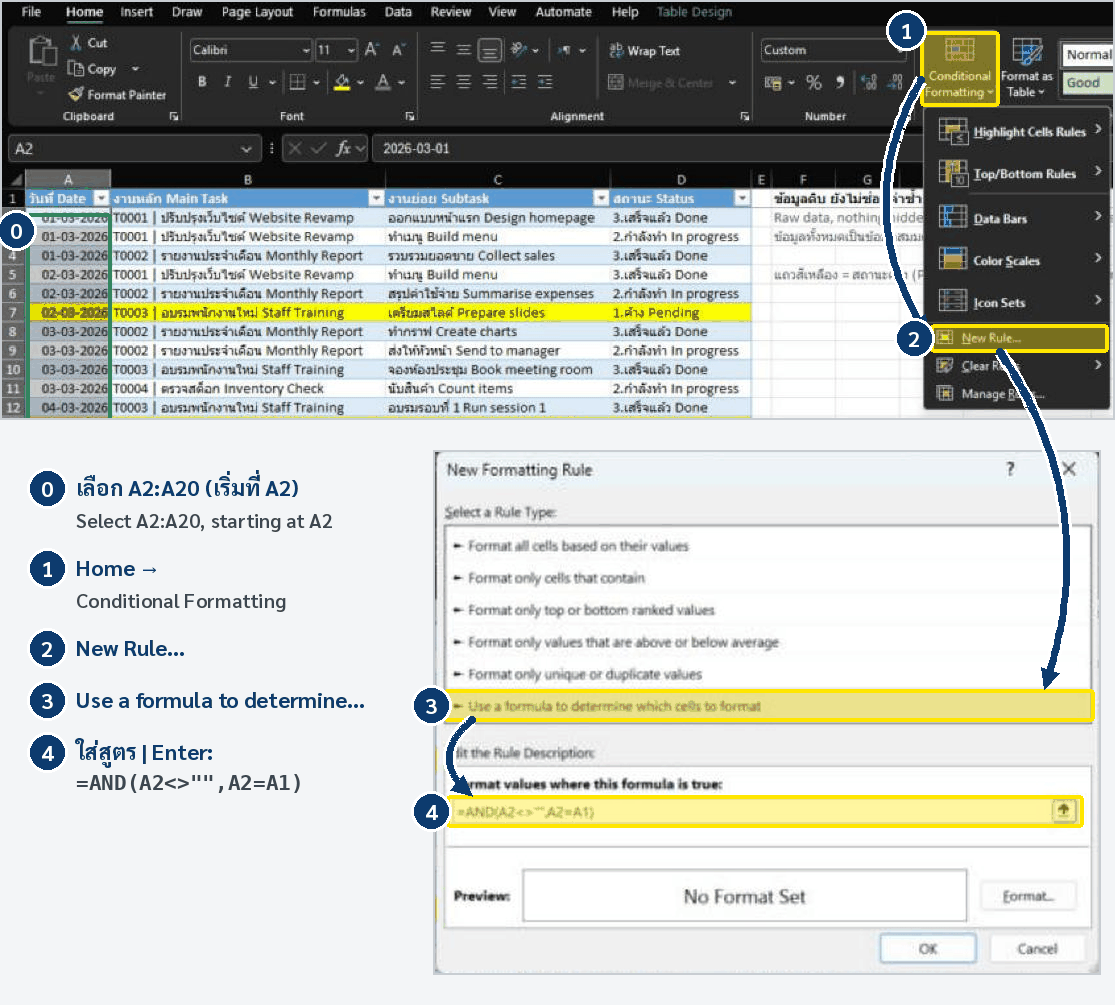
ขั้นตอน | Steps
| # | ภาษาไทย | English |
|---|---|---|
| 1 | เรียงข้อมูลตามวันที่ก่อน | Sort by Date first |
| 2 | ลากเลือก A2:A20 โดยเริ่มที่ A2 | Select A2:A20, starting at A2 |
| 3 | Home → Conditional Formatting → New Rule | Home → Conditional Formatting → New Rule |
| 4 | เลือก Use a formula to determine which cells to format | Choose Use a formula to determine which cells to format |
| 5 | ใส่สูตร =AND(A2<>"",A2=A1) | Enter =AND(A2<>"",A2=A1) |
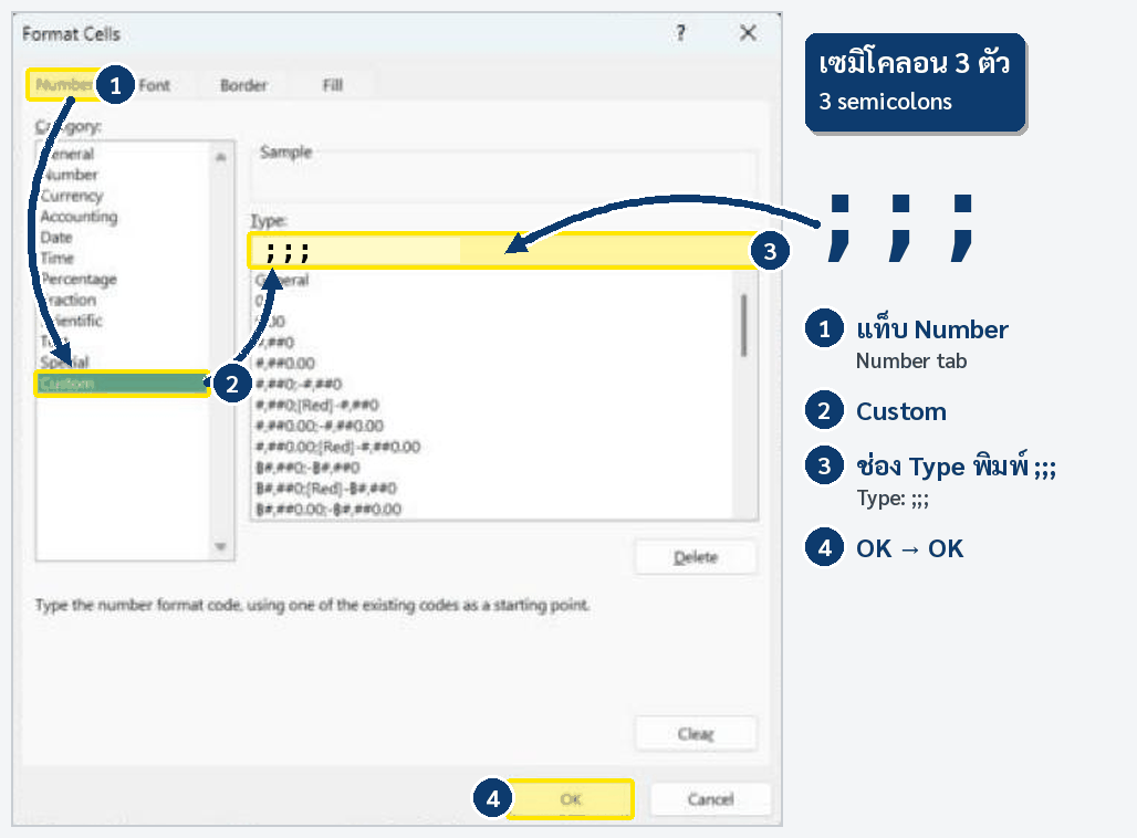
| 6 | กด Format… → แท็บ Number → Custom | Click Format… → Number tab → Custom |
| 7 | ช่อง Type พิมพ์ ;;; (เซมิโคลอน 3 ตัว) | In Type, enter ;;; (3 semicolons) |
| 8 | กด OK → OK | Click OK → OK |
ขั้นตอนที่ 5: สูตร | Step 5: formula=AND(A2<>"",A2=A1)
ขั้นตอนที่ 7: Custom number format | Step 7: custom number format;;;
สูตรนี้แปลว่าอะไร | What the Formula Means
| ส่วน Part | ภาษาไทย | English |
|---|---|---|
A2=A1 | แถวนี้เหมือนแถวบนไหม | Same as the row above? |
A2<>"" | เซลล์นี้ไม่ว่าง | The cell is not empty |
AND(...) | ซ่อนเมื่อเข้าเงื่อนไขทั้งสองข้อ | Hide only when both are true |
ทำไม ;;; ถึงซ่อนได้ | Why ;;; Works
THรูปแบบตัวเลขแบบ Custom แบ่งเป็น 4 ช่อง คั่นด้วย ; คือ บวก ; ลบ ; ศูนย์ ; ข้อความ
;;; คือไม่ใส่อะไรเลยทั้ง 4 ช่อง Excel เลยไม่แสดงอะไร ไม่ว่าพื้นจะเป็นสีอะไร
ENA custom number format has 4 parts split by ;: positive ; negative ; zero ; text.
;;; leaves all 4 empty, so Excel shows nothing, on any background.
5. ตัวอย่างที่ 2: ซ่อนชื่องานซ้ำ แต่ขึ้นใหม่เมื่อเปลี่ยนวัน | Example 2: Hide Repeated Tasks, Show Again on a New Day
THงานหลักหนึ่งงานมีงานย่อยหลายแถว เราอยากซ่อนชื่องานที่ซ้ำ
แต่ถ้าขึ้นวันใหม่ ชื่องานควรกลับมาแสดง ถึงจะเป็นงานเดิมก็ตาม
ถ้าใช้แค่ =B2=B1 ชื่องานจะหายข้ามวัน ดูแถว 5 ในตารางนี้
ENOne main task can have many subtask rows. We want to hide the repeats.
But on a new day, the task name should show again, even if it's the same task.
With only =B2=B1, the name stays hidden across days. See row 5 below.
| แถวRow | A วันที่Date | B งานหลักMain Task | =B2=B1 | =AND($A2=$A1,B2=B1) |
|---|---|---|---|---|
| 2 | 01/03 | T0001 | ปรับปรุงเว็บไซต์ | แสดง Show | แสดง Show |
| 3 | 01/03 | T0001 | ปรับปรุงเว็บไซต์ | ซ่อน Hide | ซ่อน Hide |
| 4 | 01/03 | T0002 | รายงานประจำเดือน | แสดง Show | แสดง Show |
| 5 | 02/03 | T0002 | รายงานประจำเดือน | ❌ ซ่อน Hide | ✅ แสดง Show |
| 6 | 02/03 | T0003 | อบรมพนักงานใหม่ | แสดง Show | แสดง Show |
ขั้นตอน | Steps
| # | ภาษาไทย | English |
|---|---|---|
| 1 | เรียงตาม วันที่ แล้วตาม งานหลัก | Sort by Date, then Main Task |
| 2 | ลากเลือก B2:B20 โดยเริ่มที่ B2 | Select B2:B20, starting at B2 |
| 3 | New Rule → Use a formula… | New Rule → Use a formula… |
| 4 | ใส่สูตร =AND(B2<>"",$A2=$A1,B2=B1) | Enter =AND(B2<>"",$A2=$A1,B2=B1) |
| 5 | Format → Number → Custom → ;;; → OK → OK | Format → Number → Custom → ;;; → OK → OK |
ขั้นตอนที่ 4: สูตร | Step 4: formula=AND(B2<>"",$A2=$A1,B2=B1)
ขั้นตอนที่ 5: Custom number format | Step 5: custom number format;;;
TH$A คือล็อกให้เช็กวันที่จากคอลัมน์ A เสมอ
EN$A locks the check to the Date column (column A).
THถึงวันที่ในคอลัมน์ A จะถูกซ่อนไปแล้ว สูตรก็ยังอ่านค่าได้ เพราะ ;;; แค่ซ่อนการแสดงผล ค่าจริงยังอยู่
ENEven if the dates in column A are hidden, the formula still reads them. ;;; only hides the display. The value stays.
6. ข้อควรระวัง | Watch Out
| # | ภาษาไทย | English |
|---|---|---|
| 1 | ต้องเรียงข้อมูลก่อน สูตรเทียบกับแถวบนแถวเดียว ถ้าค่าซ้ำอยู่ห่างกัน จะไม่ถูกซ่อน | Sort first. The rule only checks the row above. Repeats that are far apart won't hide. |
| 2 | สูตรต้องอ้างแถวบนของแถวแรกที่เลือก เลือกจาก A2 ต้องเขียน A2=A1 ถ้าเขียนผิดแถว จะซ่อนผิดเซลล์ | Point to the row above your first row. Start at A2 → write A2=A1. The wrong row hides the wrong cells. |
| 3 | ข้อมูลยังอยู่ครบ SUM, COUNT, XLOOKUP, Sort, Filter ใช้ได้ปกติ | The data is still there. SUM, COUNT, XLOOKUP, Sort and Filter work as normal. |
| 4 | ตอนกรอง (Filter) สูตรยังเทียบกับแถวบนที่ถูกกรองซ่อนไป แถวแรกที่เห็นอาจดูว่าง | When filtering, the rule still checks the hidden row above. The first visible row may look empty. |
| 5 | คนอื่นอาจไม่รู้ว่ามีข้อมูลซ่อนอยู่ เขียนหมายเหตุไว้ข้างตาราง | Others may not know data is hidden. Add a short note next to the table. |
| 6 | ถ้าใช้ Table กฎจะขยายเองเมื่อเพิ่มแถว แต่การ copy/paste ทับอาจทำให้กฎแตกเป็นหลายชิ้น ให้เช็กที่ Manage Rules | In a Table, the rule grows with new rows. Pasting over cells can split it. Check Manage Rules. |
| 7 | ฟีเจอร์นี้มีใน Excel บน Windows มานานแล้ว ถ้าใช้ Excel บนเว็บหรือ Mac ให้ลองก่อน | This works in Excel for Windows. On Excel for the web or Mac, test it first. |
7. เอาไปใช้ต่อได้อีก | More Ideas
| ไอเดีย Idea | สูตร Formula (เริ่มแถว 2 · start at row 2) |
|---|---|
| ซ่อนชื่อลูกค้าที่ซ้ำHide repeated customer names | =AND(B2<>"",B2=B1) |
| ซ่อนเลขใบสั่งซื้อที่ซ้ำHide repeated order numbers | =AND(C2<>"",C2=C1) |
| ซ่อนเลข 0 เฉพาะแถวที่ยกเลิกHide zeros on cancelled rows | =AND($D2="4.ยกเลิก",E2=0) |
| ซ่อนตัวเลขทั้งแถวที่ยกเลิกHide all numbers on cancelled rows | =$D2="4.ยกเลิก"(เลือกทั้งแถว · select whole rows) |
| ซ่อนหมวดหมู่ย่อยที่ซ้ำHide repeated sub-categories | =AND($A2=$A1,B2=B1) |
💡 แตะที่สูตรเพื่อคัดลอก | Tap a formula to copy it.
THทุกไอเดียใช้หลักเดียวกัน สูตรบอกว่า "ซ่อนเมื่อไหร่" แล้วให้ ;;; เป็นตัวซ่อน
ENSame idea every time: the formula says when to hide, and ;;; does the hiding.
8. ไฟล์ตัวอย่าง | Sample File
THไฟล์มี 3 ชีต ข้อมูลทั้งหมดเป็นข้อมูลสมมติ ทุกชีตเป็น Table แบบแถวสลับสี และแถวที่สถานะ "1.ค้าง Pending" ไฮไลต์สีเหลือง เพื่อให้เห็นว่าวิธีนี้ใช้ได้บนพื้นสีจริง
01_Before– ข้อมูลดิบ ยังไม่ซ่อน ไว้ฝึกทำตาม02_Dates– ตัวอย่างที่ 1: ซ่อนวันที่ซ้ำ03_MainTasks– ตัวอย่างที่ 2: ซ่อนวันที่ซ้ำ + ซ่อนชื่องานซ้ำในวันเดียวกัน
ENThe file has 3 sheets with fictional data. Each sheet is a Table with banded rows. Rows with status "1.ค้าง Pending" are highlighted yellow, so you can see the trick works on coloured rows.
01_Before– raw data, nothing hidden, for practice02_Dates– Example 1: hide repeated dates03_MainTasks– Example 2: hide repeated dates + repeated tasks within the same day
สรุปสั้นๆ | Quick Recap
THสูตร =AND(A2<>"",A2=A1) + Format → Number → Custom → ;;;
= ซ่อนค่าซ้ำ เหลือตัวแรก ใช้ได้บนพื้นทุกสี
ENFormula =AND(A2<>"",A2=A1) + Format → Number → Custom → ;;;
= hide repeats, keep the first, works on any background.